How to properly tune a PID

This article comes to summarize the fantastic video that Peter Harrison made a few days ago on YouTube about the simplest and most effective way to tune a PID in a few minutes instead of days. I followed that video to tune the LibreServo PID and the results were amazing.

There are hundreds of guides on the Internet on how to adjust a PID and they can all be summarized in the following simple steps:

• Set K_D and K_I to zero and increase K_P until the system corrects the error and starts oscillating. That would be the maximum K_P
• Increase K_D until the K_P oscillation stops.
• Increase K_I slightly so that the system fully corrects the error.

They seem like three simple and quick steps, but the reality is that in the end it becomes a sort of trying to guess the constants and after hundreds of tests and hours, if you are lucky, you get a relatively stable PID. It is a rather cumbersome task that rarely achieves a completely satisfactory result.

Let's forget about all that and try to obtain K_P and K_D mathematically. K_I in a dynamic system is not necessary on most occasions and introduces more disadvantages than advantages, so we will forget about it for now. From now on, although I talk about a PID, I am really referring to a PD.

Step one. Characterize your system/engine

This step is the most difficult, characterizing your system. Assuming you want to drive a motor, you have to have at least one motor readout system, an encoder. It doesn't matter if it is super accurate 65,000 steps like LibreServo or simple 12 steps like Pololu, but at least you have to have an encoder. If you don't have an encoder for your system, then you have no choice but to follow the above three steps. If you do have a sensor, an encoder in our case, then continue.

Let's focus on motors. To characterize a motor we have to know how its speed varies by applying one voltage or another and how fast the speed changes with voltage changes. This part should be done with a system as close to the final one as possible if we cannot do it with the real one, that is, if our motor is going to be the motor that moves a line-follower, the results will be closer to reality if they are done by moving the line-follower itself or a similar weight instead of moving the motor free.

System gain, K_m

For the first part, we measure the motor speed with a PWM of 50%. To make sure that the speed is already constant, we measure the speed after a reasonable time after applying the PWM, for example one second after. Make several measurements and make an average. In our case it gave us 10,205 encoder steps every second.

Repeat the same procedure but now with a PWM of 75%. Make several measurements of the speed and make the average. In our case it gave us 15,482 encoder steps every second.

Having the velocity at two given points, we can now obtain the gain of the system. The gance is linear, and therefore fits the formula y = mx + b. So substituting we obtain:
10.205 = m*50 + b
15.482 = m*75 + b
The result is: y = 211x - 345. Therefore, the gain of the system (K_m) is 211.

Time constant of the system, T_m

For the second part, we are not interested in the speed the motor reaches, but how fast it reaches it. To do this, with a PWM at 50% of which we know the speed the motor reaches, we measure the acceleration ramp of the motor and see at what point it reaches 63% of its speed for that 50% PWM. In our case the motor takes 16ms to reach the speed of 6,429, 63% of 10,205.

There is no need to repeat this second step with a PWM at 75%, as it should give the same result. Even so, it can be repeated to make sure we are on the right track.

In the following picture I show this same process that I did for LibreServo where you can see graphically what I said:

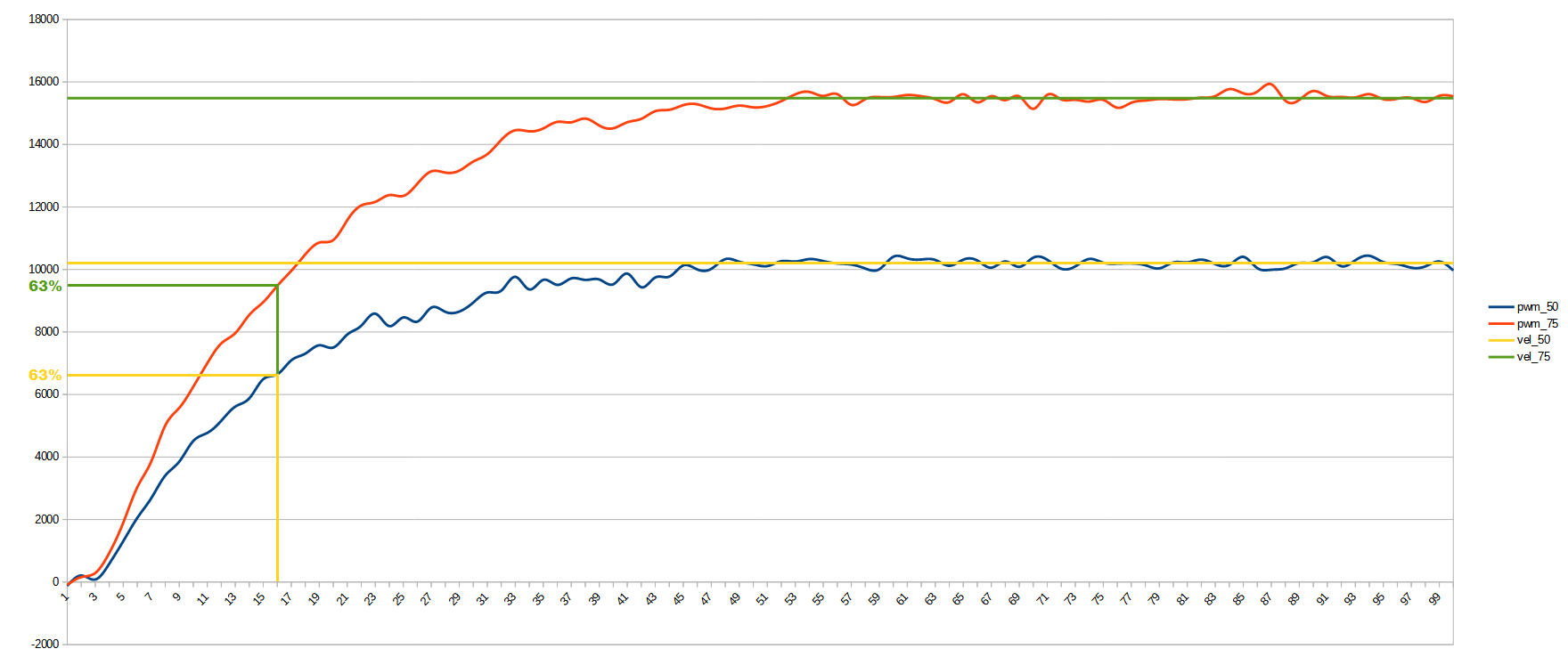Engine response graph

Second step. Calculate K_P and K_D

We have already calculated K_m and T_m which are 211 and 0.016 respectively in our case, now only the simple part remains. But before continuing we must mention the damping variable, or ζ.

Damping variable ζ

Without going into details, the damping variable or ζ (Zeta), affects the response of a second order system to a change. What we need to know about this variable (which we will use later), is that any value greater than zero will make the system stable sooner or later. One (1) is the first value of ζ at which there is no overshoot in the system, higher values make the system slower. Lower values make it reach the target value faster but with overshoot. The ζ value of 0.707 is the fastest value at which the system reaches the target value and does not overrun by more than 5%. This value, 0.707 is usually the value chosen for ζ.

In the following image courtesy of sumemura.jp, we can see graphically what has been said so far:

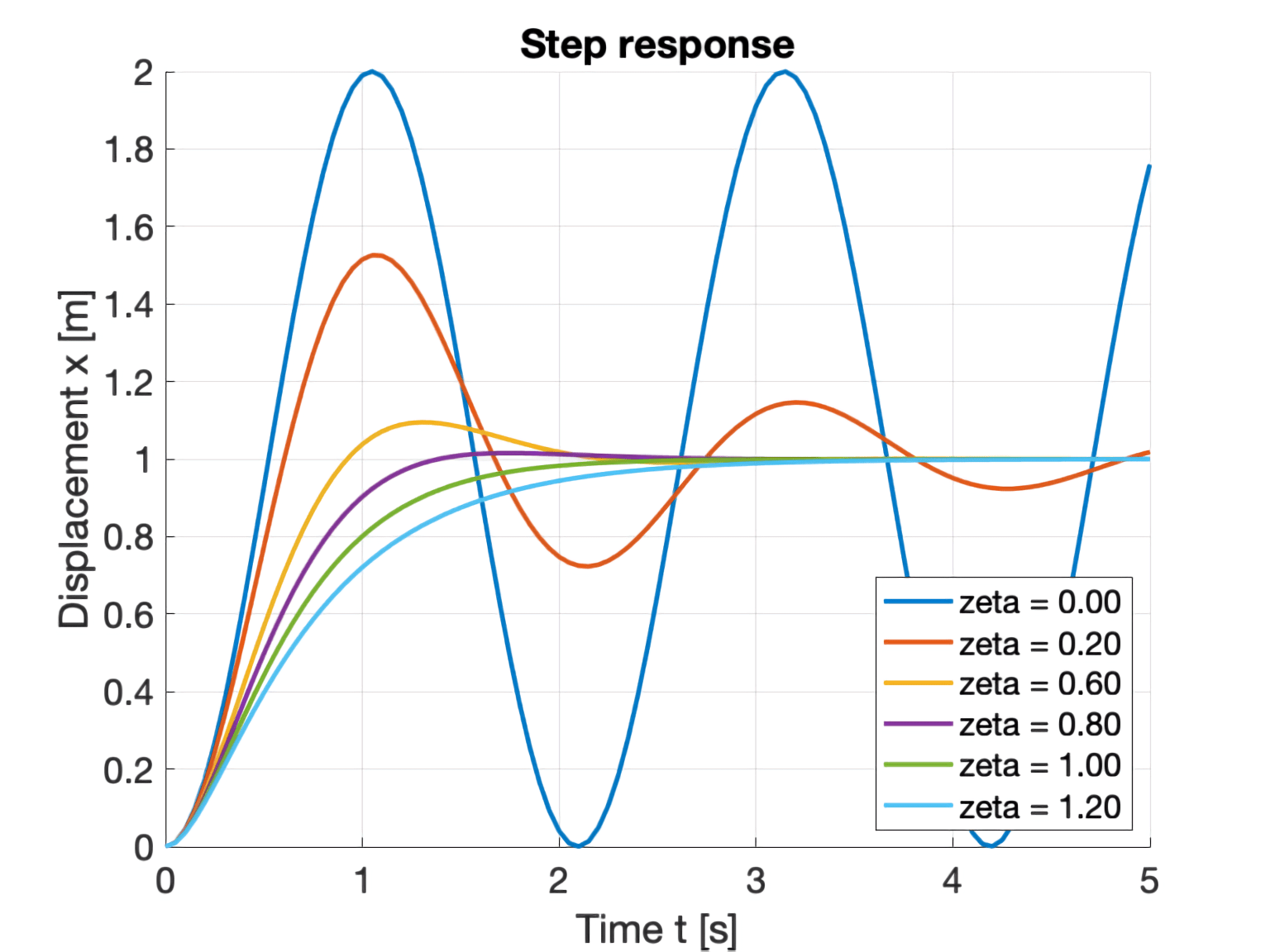Step response of a second-order system

Calculation of K_P and K_D

We will now calculate the variables K_P and K_D. For this we will use the following two formulas:
K_P = T_m⁄K_m · 16⁄ζ²T²_D
K_D = 8T_m-T_D⁄T_DK_m

It may seem very complex, but we already have all the variables except T_D, stabilization time. For this, a good value to start with would be the same as T_m or half of it. If we use half, the formulas in our case would be:K_P = 0,016⁄211 · 16⁄0.707²0,008² = 38
K_D = 8·0,016-0,008⁄0,008·211 = 0,1469
We multiply the value of K_D by the frequency of our PID, 4KHz, giving us a value of 284. That will be the value to substitute in our PID code.

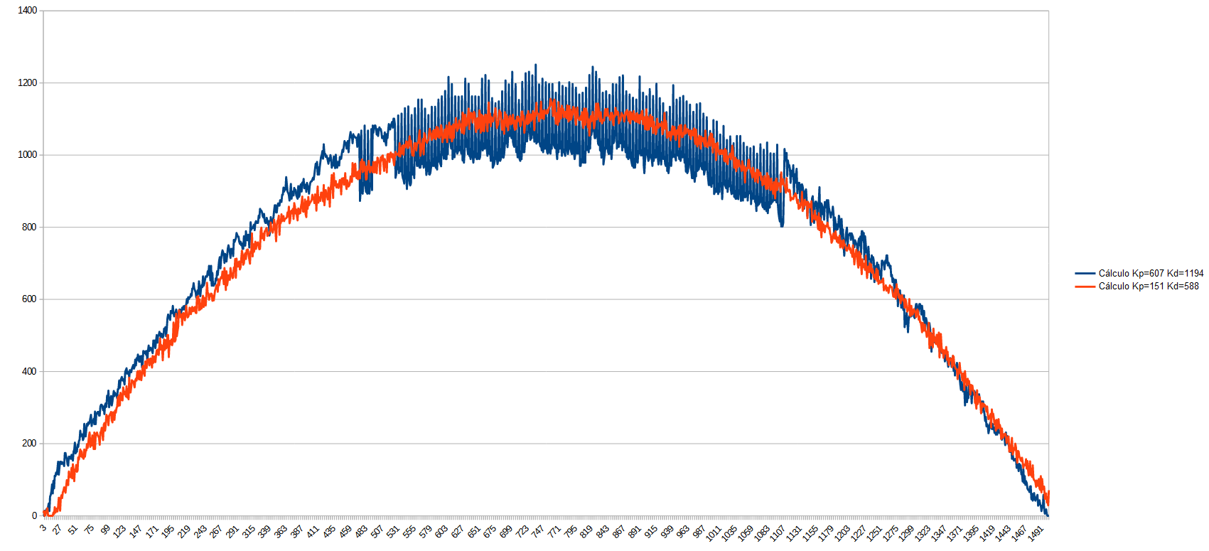
The following graph shows the response of the LibreServo engine with the values that I had obtained manually, and that I noticed that I had to continue optimizing, and the response with the new calculated values. The motor tries to follow a hermitic curve, which is perfect to see how it behaves at different speeds:

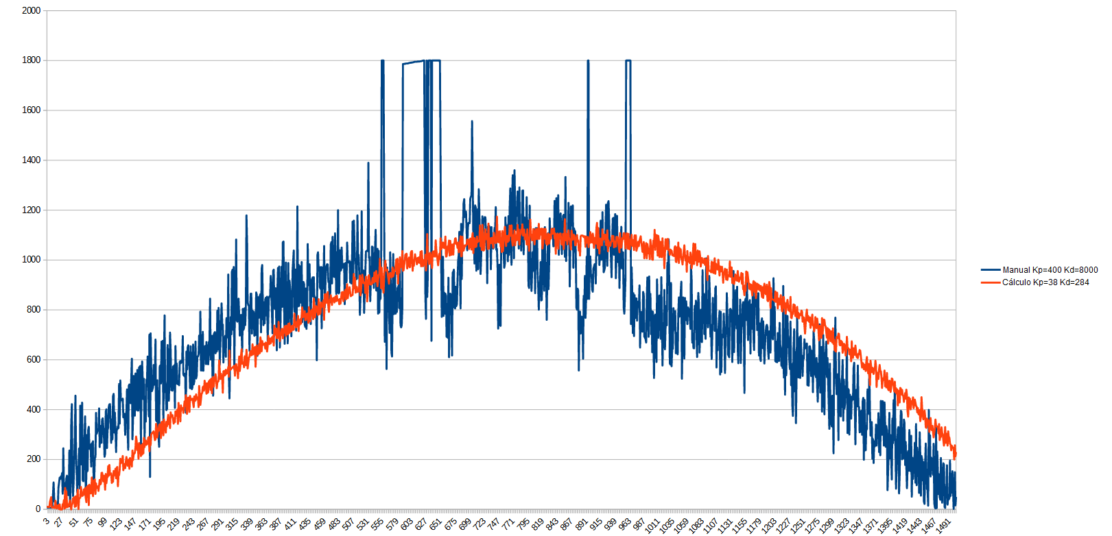Comparison of the PWM in the motor with different PIDs

We see that the original PID saturated the motor in several situations, and although it correctly followed the motion curve, that control was very harmful to the mechanics of the motor, instead, with the new calculated values, we have achieved an almost ideal control at the first time. We see that it has a certain delay in the response, so let's reduce T_m to 0.004:

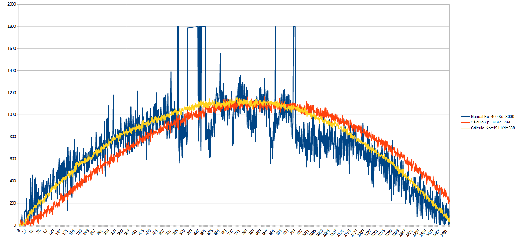Comparison of the PWM in the motor with different PIDs

Now we have achieved a practically perfect response in just two attempts and a few minutes. But what happens if we reduce T_m even further? Let's see what happens when we reduce T_m even further, for example to 0.002:

Comparison of the PWM in the motor with different PIDs

Now we see that reducing too much T_m causes that the control is no longer so effective and noises start to appear, therefore, we stay with the previous PID.

In the following video we can notice the sound of the servomotor. The movement is the same, but with one PID the motor sound is not correct and with the second PID we hear something much more natural and correct.

LibreServo Specific Considerations

In the case of LibreServo, a small distinction is added between the PID during a movement and the PID in static, maintaining a position. During the movement the PID will actually be a PD, but in static the PID changes and the integral part is added, this is done to ensure that in any circumstance and load the servomotor maintains its position and in many cases finish centering the final position.